Peptide Half-Lives Explained: How They Determine Dosing Frequency

First-Order Elimination and Why It Applies to Research Peptides

When a compound leaves the body, the rate at which it disappears is not constant. It does not eliminate at the same speed regardless of how much is present. Instead, for most small peptides under research conditions, the elimination rate is proportional to the current concentration: the more that is present, the faster it clears. This is called first-order kinetics, and it is the standard model for research peptide pharmacology.

The mathematical implication is elegant: the concentration at any point in time equals the starting concentration multiplied by e raised to the power of negative k times t, where k is the elimination rate constant and t is time elapsed. That rate constant k equals the natural logarithm of 2 divided by the half-life. This is why half-life is the single most practically useful pharmacokinetic parameter for research protocol design. It encapsulates the entire elimination behaviour in one number.

First-order elimination means that each successive half-life removes exactly half of whatever remains. Start with 100 units, and after one half-life you have 50. After two half-lives, 25. After three, 12.5. The exponential decay curve is smooth and predictable, which is what makes the five-half-life rule so reliable.

The Five-Half-Life Rule for Reaching Steady State

When a peptide is dosed repeatedly at a fixed interval, the body is simultaneously eliminating what was given previously while accumulating what is being given now. Initially, these two processes are not in balance: concentration rises with each administration. Over time, however, the rate of elimination catches up to the rate of administration, and the system reaches an equilibrium. This equilibrium is called steady state.

The practical benchmark is five half-lives. After five half-lives of repeated dosing, the trough concentration (the lowest point in each dosing interval) has reached more than 96.9% of its eventual steady-state value. For most research purposes, this is considered equivalent to full equilibrium.

The implication for protocol design is significant. A researcher who begins a protocol and expects to measure representative responses in week one is measuring the induction phase, not steady-state behaviour. Any endpoint that depends on consistent plasma levels must be assessed after the five-half-life threshold has been crossed.

Accumulation Factor: Predicting the Trough-to-Peak Ratio

The accumulation factor quantifies how much the trough concentration at steady state exceeds the concentration after a single dose. It is calculated as 1 divided by the quantity 1 minus e to the power of negative k times the dosing interval. For a peptide with a very short half-life dosed daily, k is large, the exponential term approaches zero, and the accumulation factor approaches 1, meaning no accumulation. For a peptide with a long half-life dosed at the same or shorter interval, the accumulation factor grows considerably.

The accumulation factor matters for two reasons. First, it tells a researcher how much more peptide will be present at steady state compared to after the first dose, which affects the interpretation of any measurement taken early in the protocol. Second, it determines the peak-to-trough fluctuation ratio: how much concentrations swing between doses. A high accumulation factor with stable concentrations is generally more desirable for protocols requiring consistent effect levels. A low accumulation factor means every dose is essentially starting from near-zero, which suits protocols designed to study acute pulsatile responses.

Short Half-Life Peptides: No Accumulation

Tesamorelin has a half-life of approximately 24 minutes. CJC-1295 in its non-DAC form (also called Mod GRF 1-29) has a half-life of around 30 minutes. Both are GHRH analogs dosed daily or multiple times daily.

For a peptide with a 30-minute half-life dosed once every 24 hours, the dosing interval is 48 times the half-life. By the time the next dose is administered, the previous dose has been reduced to an infinitesimal fraction of its original concentration, less than one part in 281 trillion, mathematically. In practice, it has been eliminated entirely. The accumulation factor is essentially 1. Every administration is pharmacologically independent.

This means the steady-state concept, while technically still valid, is practically irrelevant for short half-life peptides on daily schedules. There is no meaningful accumulation to model and no trough elevation to consider. The response window is brief and closely coupled to the administration event. Protocols studying these peptides are studying acute pulsatile effects, and data collection should be timed accordingly.

Long Half-Life Peptides: Accumulation Factor Near 2

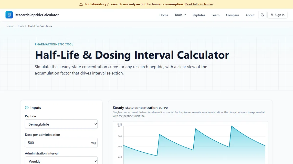
Semaglutide has a half-life of approximately 168 hours (seven days). On a weekly dosing schedule, the dosing interval equals exactly one half-life. At this ratio, the accumulation factor is 2. Steady-state trough concentration is double the concentration seen after the first dose. Steady state is reached after approximately five weeks of weekly administration.

Tirzepatide has a half-life of roughly 120 hours, meaning its dosing interval is 1.4 half-lives on a weekly schedule and its accumulation factor is somewhat lower than semaglutide's, but still substantially above 1. A researcher measuring glycaemic or metabolic responses in week two of a tirzepatide protocol is not measuring steady-state responses — they are measuring sub-steady-state responses that may not reflect the compound's full effect profile.

This is not a minor point for titration design. The common practice of beginning at a low dose for tolerability and escalating stepwise means the subject progresses through each dose level before that level reaches steady state. Titration cadence (typically four weeks per step in major incretin trials) must accommodate this accumulation timeline. Plot steady-state concentration curves for any peptide half-life to visualise how quickly any given compound reaches equilibrium on a chosen schedule.

Dosing Interval Relative to Half-Life: Shaping Peak-to-Trough Fluctuation

The ratio of dosing interval to half-life is the variable that controls fluctuation. When this ratio is small (when the dose is administered much more frequently than every half-life), concentrations remain relatively flat between doses. When the ratio is large (dosing every several half-lives), concentrations rise sharply after each dose and fall substantially before the next.

For incretins with weekly schedules and multi-day half-lives, the daily concentration profile is relatively smooth despite once-weekly dosing. This is by design: the long half-lives of semaglutide and tirzepatide were engineered specifically to enable weekly administration with minimal fluctuation.

For GH-axis peptides with 30-minute half-lives, the fluctuation is extreme by comparison. A single pulse produces a sharp concentration spike that disappears within hours. Whether this mirrors physiological GH release patterns — which are themselves pulsatile — is part of the rationale for their use in research. The relationship between half-life and dosing interval is therefore not just a pharmacokinetic curiosity; it is a design choice with direct implications for what any given protocol actually measures.

Practical Implications for Titration Schedules

Steady-state thinking transforms how researchers approach titration design. If the goal is to assess tolerability at a given dose level before escalating, the assessment should take place after that level has had time to reach steady state. For a weekly-dosed incretin with a five-day half-life, that means allowing at least five weeks at each dose level before drawing conclusions. The major trial protocols (STEP for semaglutide, SURMOUNT for tirzepatide) were structured with exactly this logic in mind, using four-week minimum steps even during the escalation phase.

For the in-depth reference on understanding peptide half-lives, the underlying mathematics and worked examples for additional compounds are documented in detail. Building half-life awareness into protocol design from the outset is the difference between collecting data that answers a defined question and collecting data that describes a system still finding its equilibrium.